Validation
Compression is only useful if we can say clearly what it preserves and what it changes.
For that reason, step2point separates validation into two categories.
Quantities that should stay unchanged
These are the observables that define whether the compressed shower still behaves like the original shower.
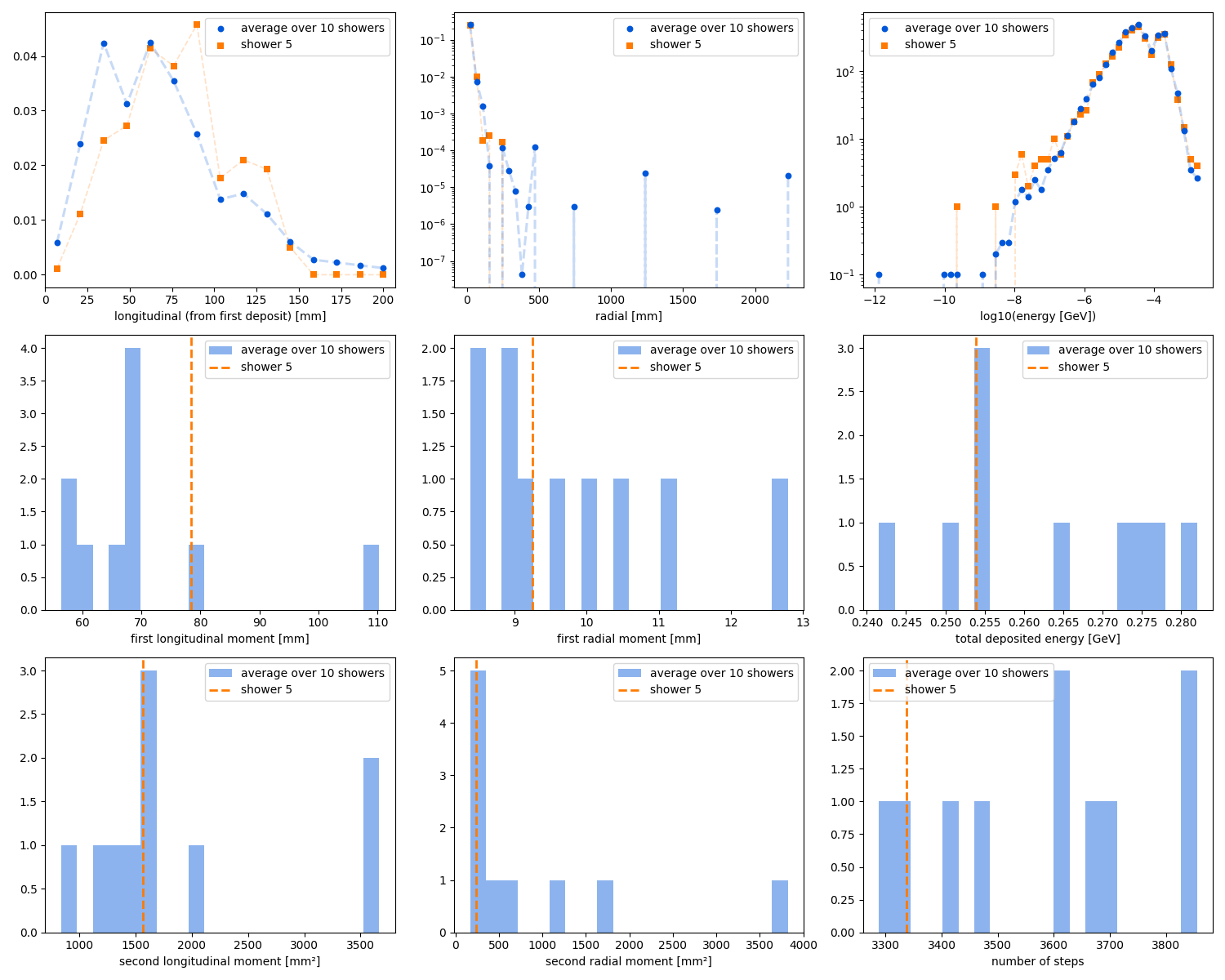
Total shower energy
A natural diagnostic is the per-shower ratio:
E_post / E_pre
Using a ratio is usually more informative than looking at raw energies directly, because it factors out the broad physical energy range in the dataset.
Shower profiles
The compressed shower should preserve the broad shape of the shower:
- longitudinal profile
- radial profile
- phi profile
Shower moments
Useful compact summaries are:
- first longitudinal moment
- second longitudinal moment
- first radial moment
- second radial moment
Detector-aware quantities
If cell_id is present, detector-aware checks become especially important:
- distribution of
log(cell_energy) - ratio of the number of cells before and after compression
Quantities that are expected to change
Some changes are not only acceptable but are the whole point of compression.
Point-energy spectrum
The distribution of individual point energies will change because points are being merged.
Number of points
The ratio
N_points_post / N_points_pre
is one of the central performance indicators of a compression algorithm.
Example inspection workflow
For shower inspection, use examples/inspect_showers.py. The script always produces a dataset-level observables, and it also produces single-shower plots if --shower-index is given.
Note:
PYTHONPATH=src is only needed when running directly from a source checkout without installing the package first. If you already ran pip install -e .[dev], you can drop that prefix and use python ... directly.
Dataset-level only:
PYTHONPATH=src python examples/inspect_showers.py \
  --input tests/data/ODD_gamma_10ev_theta90deg_phi0deg_posX0mmY1250mmZ0mm_10GeV.h5 \
  --axis 0 1 0 \
  --outdir outputs/inspect_gamma
Dataset plus single-shower plots:
PYTHONPATH=src python examples/inspect_showers.py \
  --input tests/data/ODD_gamma_10ev_theta90deg_phi0deg_posX0mmY1250mmZ0mm_10GeV.h5 \
  --shower-index 0 \
  --axis 0 1 0 \
  --outdir outputs/inspect_gamma
Recommended axis override for these front-face ODD samples:
PYTHONPATH=src python examples/inspect_showers.py \
  --input tests/data/ODD_gamma_10ev_theta90deg_phi0deg_posX0mmY1250mmZ0mm_10GeV.h5 \
  --shower-index 0 \
  --axis 0 1 0 \
  --outdir outputs/inspect_gamma
Expected outputs:
dataset_observables.pngshower_<id>_projections.pngshower_<id>_distributions.pngshower_<id>_overview.png
Detector cell inspection
For detector-aware debugging of merging strategies, use examples/plot_detector_cells.py.
This workflow reads the DD4hep compact XML and factory-derived barrel geometry (Open Data Detector-like PolyhedraBarrel), then optionally overlays a shower from HDF5 or EDM4hep ROOT on top of:
- module envelopes
- layer outlines
- cell footprints
Typical use, to see the entire detector:
PYTHONPATH=src python examples/plot_detector_cells.py \
  --compact-xml ../OpenDataDetector/xml/OpenDataDetector.xml \
  --collection ECalBarrelCollection \
  --draw-modules \
  --overlay-input tests/data/ODD_gamma_10ev_theta90deg_phi0deg_posX0mmY1250mmZ0mm_10GeV.h5 \
  --overlay-shower-index 0 \
  --outdir outputs/detector_cells
Zoomed cell view for one module:
PYTHONPATH=src python examples/plot_detector_cells.py \
  --compact-xml ../OpenDataDetector/xml/OpenDataDetector.xml \
  --collection ECalBarrelCollection \
  --draw-cells \
  --overlay-input tests/data/ODD_gamma_10ev_theta90deg_phi0deg_posX0mmY1250mmZ0mm_10GeV.h5 \
  --overlay-shower-index 0 \
  --outdir outputs/detector_cells \
  --module 10
Zoomed view with cells spanning only over the sensitive material:
PYTHONPATH=src python examples/plot_detector_cells.py \
  --compact-xml ../OpenDataDetector/xml/OpenDataDetector.xml \
  --collection ECalBarrelCollection \
  --draw-cells \
  --sensitive-only \
  --overlay-input tests/data/ODD_gamma_10ev_theta90deg_phi0deg_posX0mmY1250mmZ0mm_10GeV.h5 \
  --overlay-shower-index 0 \
  --outdir outputs/detector_cells \
  --module 10
Manual ranges can be controlled separately for:
- axes only:
--xlim-axis--ylim-axis--zlim-axis- overlay-point selection only:
--xlim-points--ylim-points--zlim-points
Example with separate view crop and point filtering:
PYTHONPATH=src python examples/plot_detector_cells.py \
  --compact-xml ../OpenDataDetector/xml/OpenDataDetector.xml \
  --collection ECalBarrelCollection \
  --draw-cells \
  --sensitive-only \
  --overlay-input tests/data/ODD_gamma_10ev_theta90deg_phi0deg_posX0mmY1250mmZ0mm_10GeV.h5 \
  --overlay-shower-index 0 \
  --outdir outputs/detector_cells \
  --module 10 \
  --xlim-axis -7.65 7.65 \
  --ylim-axis 1307 1319 \
  --zlim-axis -7.65 7.65  \
  --xlim-points -7.65 7.65 \
  --ylim-points 1307 1319 \
  --zlim-points -7.65 7.65
There is also a --debug flag that allows to print the decoded cell ID bitfields to investigate visually the compression algorithms:
PYTHONPATH=src python examples/plot_detector_cells.py \
  --compact-xml ../OpenDataDetector/xml/OpenDataDetector.xml \
  --collection ECalBarrelCollection \
  --draw-cells \
  --sensitive-only \
  --overlay-input tests/data/ODD_gamma_10ev_theta90deg_phi0deg_posX0mmY1250mmZ0mm_10GeV_merge_within_cell_reference.h5 \
  --overlay-shower-index 0 \
  --outdir outputs/detector_cells \
  --module 10 \
  --xlim-axis -2.55 2.55 \
  --ylim-axis 1307 1319 \
  --zlim-axis -2.55 2.55  \
  --xlim-points -2.55 2.55 \
  --ylim-points 1307 1319 \
  --zlim-points -2.55 2.55 \
  --debug
The views below are all XY projections:
Module envelopes with shower overlay
Module 10 cell view with shower verlay
Module 10 sensitive-only cell view (zoomed-in) for input file

Module 10 sensitive-only cell view (zoomed-in) for merge_within_cell compression
Units used in the plots
The example HDF5 files in this repository are produced by step2point dataset repository, which preserves the EDM4hep values directly:
- deposited energy is plotted as
GeV - time is plotted as
ns - positions and shower-shape coordinates are plotted as
mm
NOTE: This matters only for axis labels and interpretation of the plots. The reclustering/compression code itself does not assume a special unit system: it preserves the units present in the input arrays. If an input dataset used different but internally consistent units, the compressed output would remain in the same units.
Validation results
EM showers
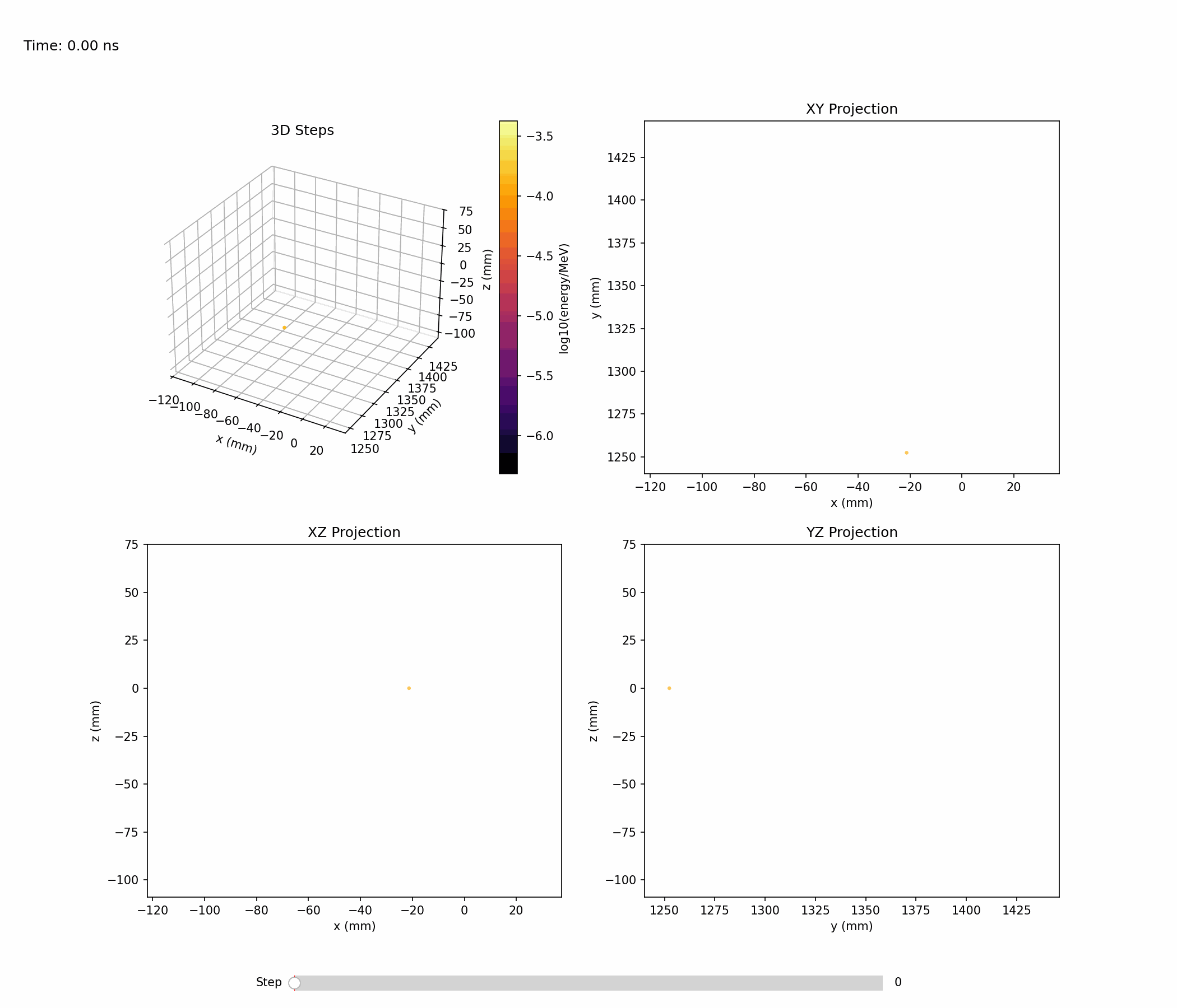
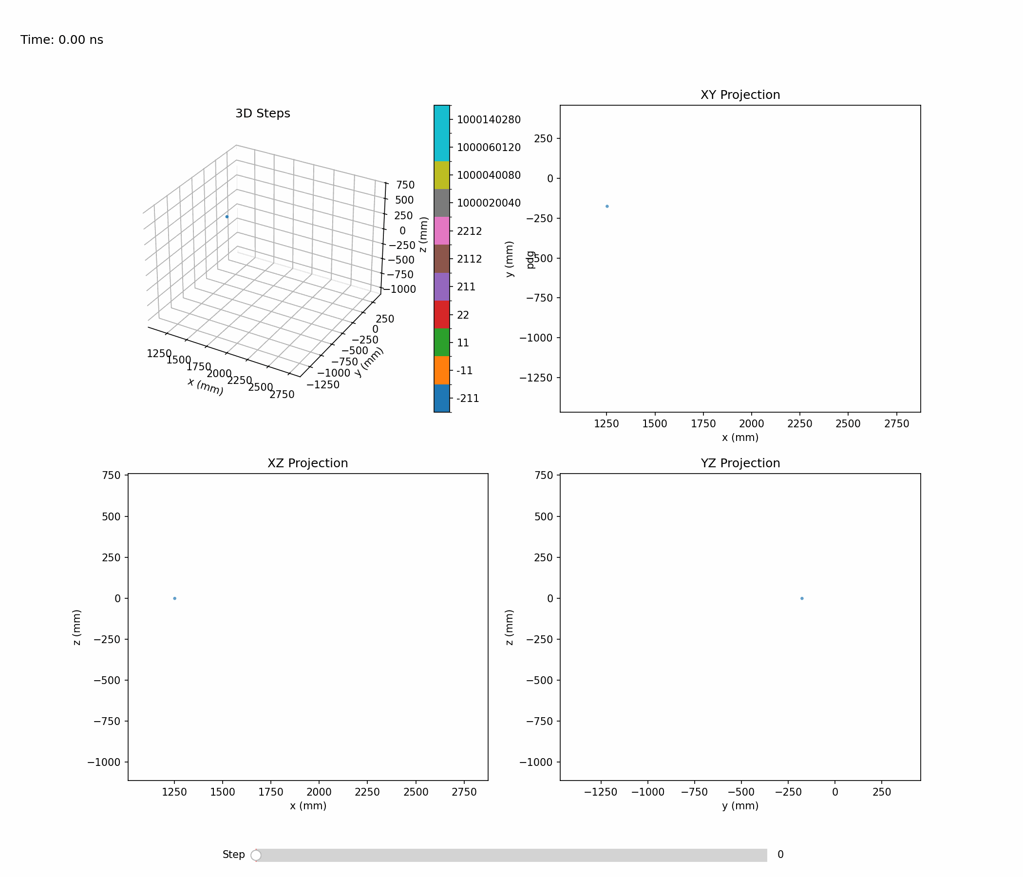
Animation below shows an example of a single electromagnetic shower:
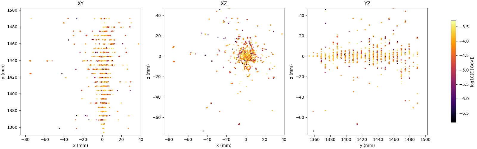
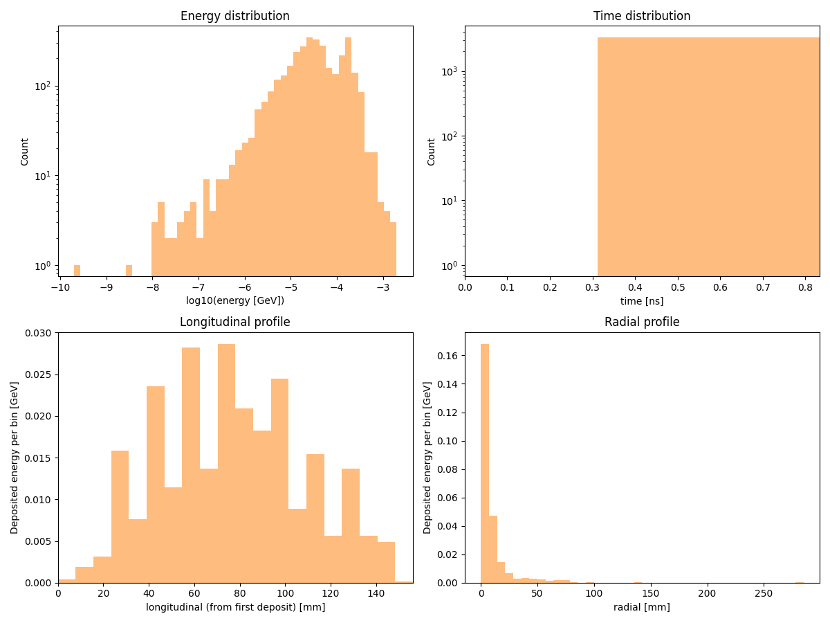
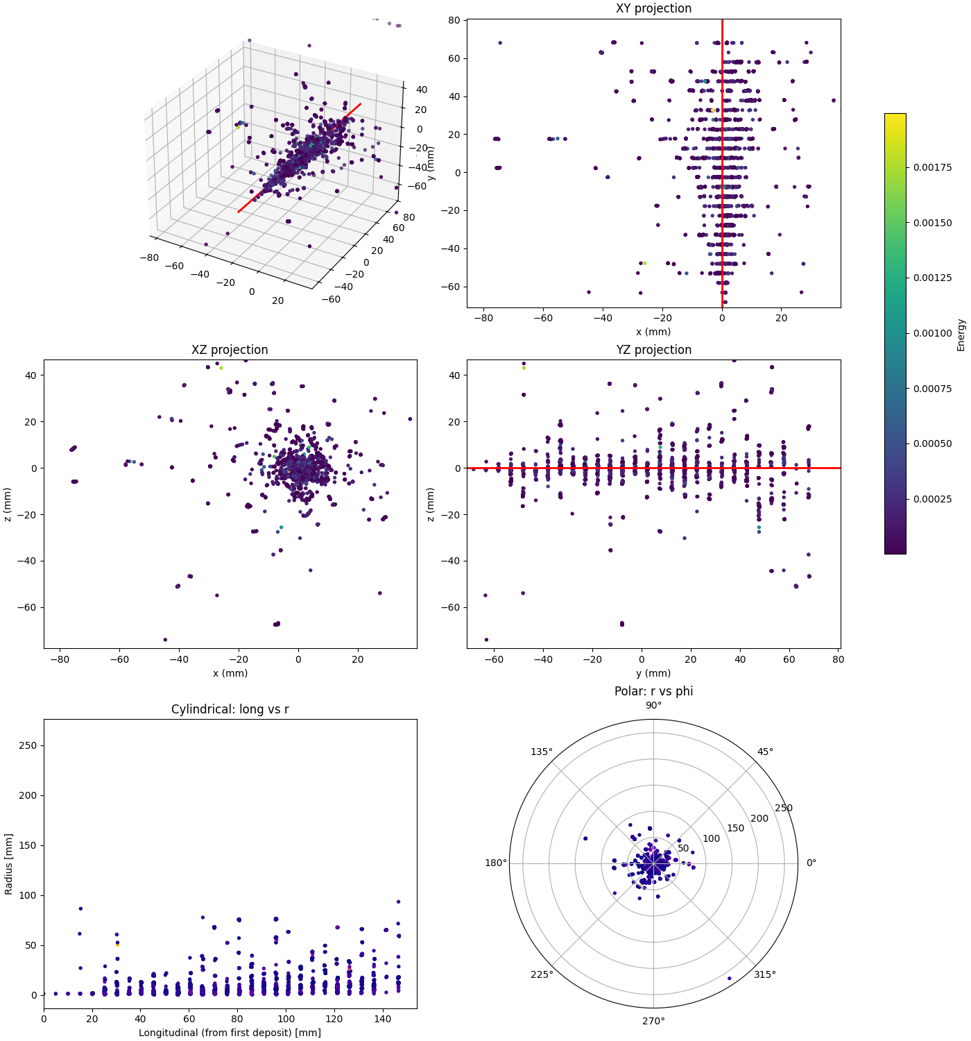
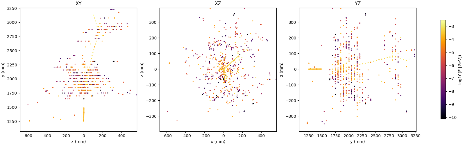
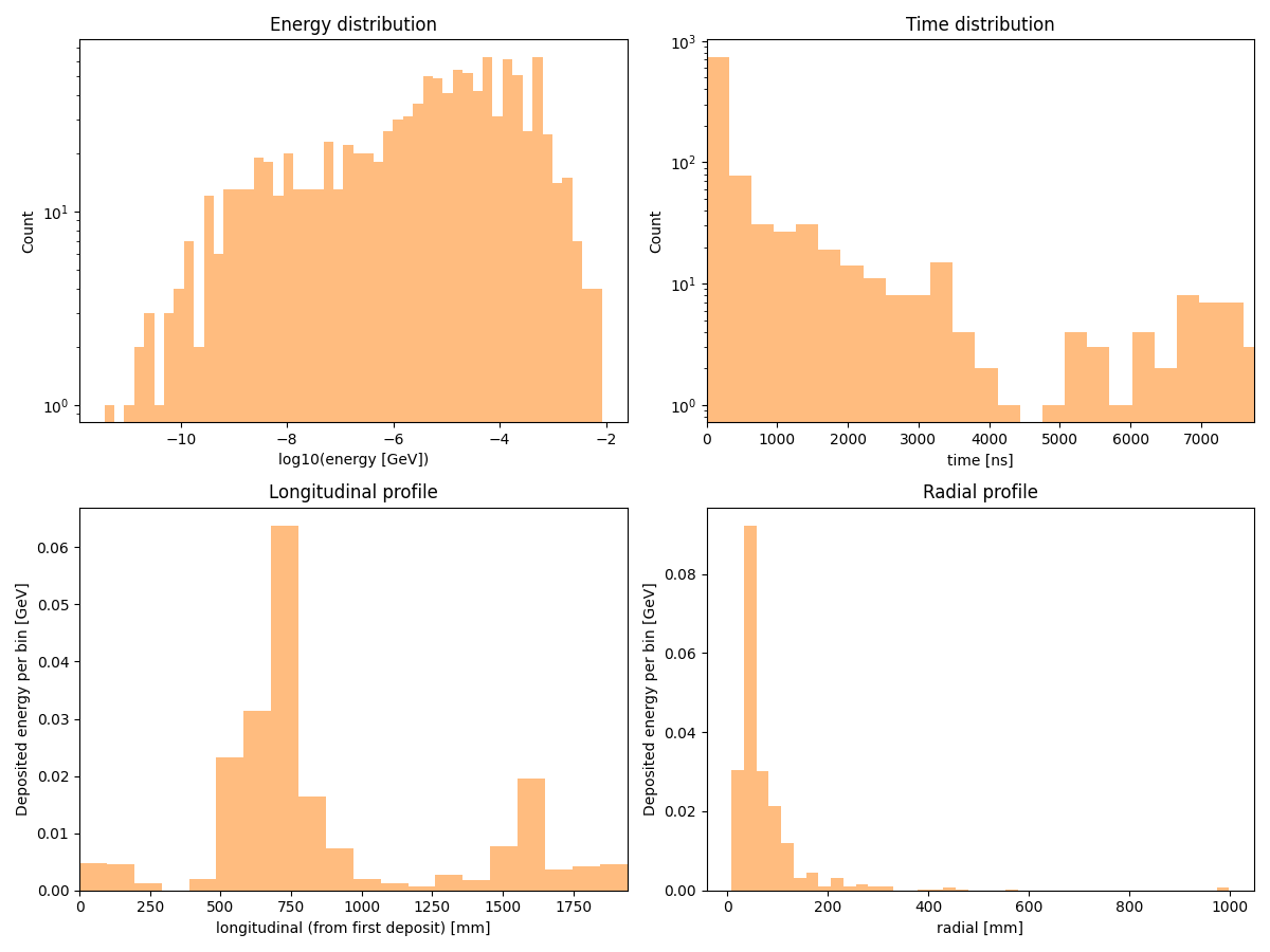
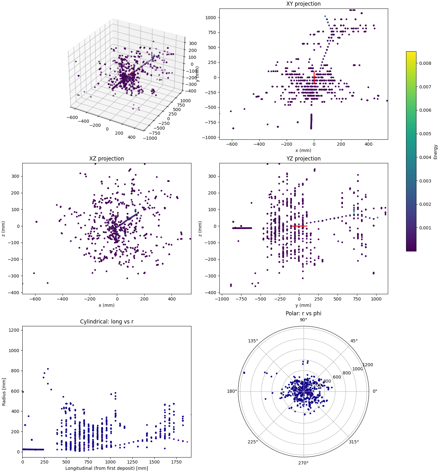
Single-shower inspection outputs produced with --shower-index 0 on the gamma sample:
Projections
Distributions
Overview
Dataset observables matrix
hadronic showers
Animation below shows an example of a single hadronic shower:
Single-shower inspection outputs produced with --shower-index 0 --axis 0 1 0 on the pion sample:
Projections
Distributions
Overview
Dataset observables